Fluid Mechanics. Bernoulli S Principle and Equation of Continuity

Fluid Mechanics. Bernoulli’s Principle and equation of continuity

EXERCISE 5

Fluid mechanics, Bernoulli’s principle

and equation of continuity

6.1. Introduction

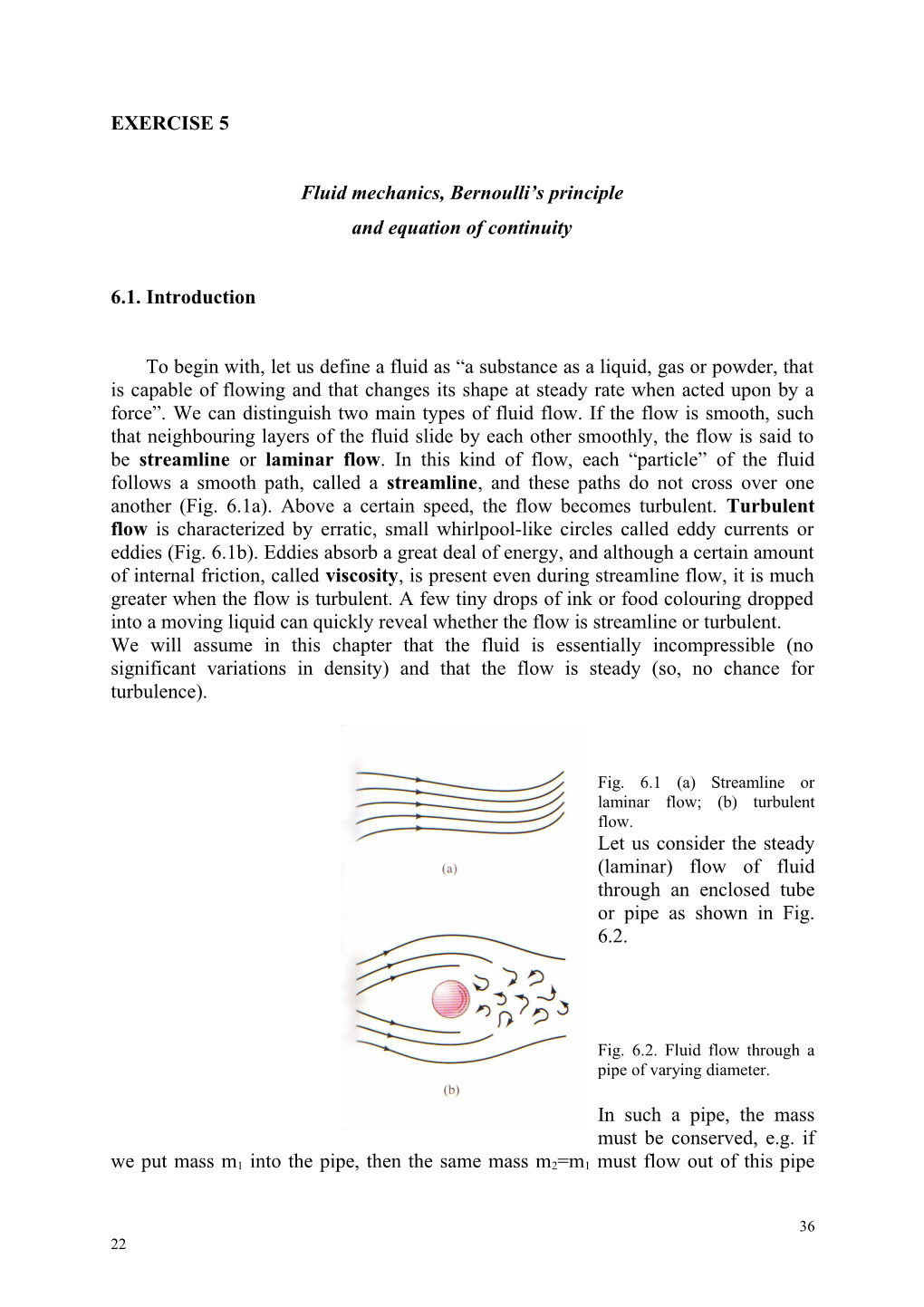
To begin with, let us define a fluid as “a substance as a liquid, gas or powder, that is capable of flowing and that changes its shape at steady rate when acted upon by a force”. We can distinguish two main types of fluid flow. If the flow is smooth, such that neighbouring layers of the fluid slide by each other smoothly, the flow is said to be streamline or laminar flow. In this kind of flow, each “particle” of the fluid follows a smooth path, called a streamline, and these paths do not cross over one another (Fig. 6.1a). Above a certain speed, the flow becomes turbulent. Turbulent flow is characterized by erratic, small whirlpool-like circles called eddy currents or eddies (Fig. 6.1b). Eddies absorb a great deal of energy, and although a certain amount of internal friction, called viscosity, is present even during streamline flow, it is much greater when the flow is turbulent. A few tiny drops of ink or food colouring dropped into a moving liquid can quickly reveal whether the flow is streamline or turbulent.

We will assume in this chapter that the fluid is essentially incompressible (no significant variations in density) and that the flow is steady (so, no chance for turbulence).

Fig. 6.1 (a) Streamline or laminar flow; (b) turbulent flow.

Let us consider the steady (laminar) flow of fluid through an enclosed tube or pipe as shown in Fig. 6.2.

Fig. 6.2. Fluid flow through a pipe of varying diameter.

In such a pipe, the mass must be conserved, e.g. if we put mass m1 into the pipe, then the same mass m2=m1 must flow out of this pipe (provided, the fluid is incompressible, since otherwise the pipe can accumulate some mass, with no outgoing flow).

Consider infinitely small portion of mass, dm, put in a time dt into the pipe. From mass conservation, we write

(6.1)

Knowing the relation of mass to volume and density, this reveals

(6.2)

Volume, that falls into the pipe in a time dt is equal V=Adx, where A is the area of cross section of the pipe, and dx is the thickness of the mass layer, pumped in time dt. Substituting this to above equation, keeping in mind the definition of velocity, we have

(6.3)

This is the continuity equation for a fluid.

Equation (6.3) tells us that where the cross-sectional area is large the velocity is small, and where the area is small the velocity is large. That this is reasonable can be seen by looking at a river. A river flows slowly through a meadow where it is broad, but speeds up to torrential speed when passing through a narrow gorge.

Have you ever wondered why smoke goes up a chimney, why a car’s convertible top bulges upward at high speeds or how a sailboat can move against the wind? There are examples of a principle worked out by Daniel Bernoulli (1700-1782) in the early eighteenth century. In essence, Bernoulli’s principle states that where the velocity of a fluid is high, the pressure is low.

Fig. 6.3 Fluid flow: for derivation of Bernoulli’s equation.

Bernoulli developed an equation that expresses this principle quantitatively. To derive Bernoulli’s equation, we assume the flow is steady and laminar the fluid is incompressible, and the viscosity is small enough to be ignored. To be general, we assume the fluid is flowing in a tube of nonuniform cross section that varies in height above some reference level, Fig 6.3.

Bernoulli’s equation in such a system is simply an expression of the work-energy theorem. What is the energy of the fluid at some position in the pipe? It is a sum of kinetic energy, potential gravitational energy, and internal energy, put by external force. For a mass element dm=ρAdx, we can write this as

(6.4.)

(6.5.)

(6.6.)

(6.7.)

The energy components have self-explanatory meaning, kinetic energy is defined as usual, gravitational potential energy also. A comment needs only be done on the internal energy. To put the mass element dm into the pipe, we have to overcome some pressure p, that exists in that pipe. This pressure generates a force , that resists the motion. Moving by dx, a work needs to be done on the fluid, . This work changes to the internal energy of the fluid.

We can divide the energy equation by dV to obtain the Bernoulli equation, which states, that the energy of a fluid doesn’t change in the flow. This is reasonable, since no energy is put to the fluid anywhere else, than in its input. Thus we have, keeping in mind that dm=ρdV, that

(6.8)

or equivalently, taking two points in the pipe and evaluating above equation for both of them,

(6.9)

This is Bernoulli’s equation. [Note that if there is no flow (v1=v2=0), then eq. (6.9) reduces to the hydrostatic equation: P2-P1=-ρg(y2-y1).]

6.2. Measurements

To begin with you have to disconnect the base from the water tap, and with help of slide calliper, measure the diameter of two cross sections (1 and 2, see the Fig. 6.4) of the tube.

Fig. 6.4. Experimental setup.

From equation of continuity and Bernoulli’s equation we can express the velocity at cross section 2 as:

(6.10)

(6.11)

(6.12)

(6.13)

(6.14)

where

-∆p=-(p2-p1)=p1-p2 is equal the hydrostatic pressure of a liquid measured by the ”Venturi tube manometer” i.e.

(6.15)

where: ρm – is the density of manometric liquid

h – is the height difference between two arms of manometer.

So, finally we can write

(6.16)

Another way of calculating v2 is by means of measuring the volume of water flowing out of tube over certain timet

(6.17)

or

(6.18)

The data should be collected in a table 6.1

Table 6.1

6.3. Results, calculations and uncertainty.

1.From the data collected in Table 6.1 calculate the average values of

(6.19)

and

(6.20)

Estimate the uncertainty of the measured values of velocities by calculating the total differential of eqs. 6.16 and 6.18 respectively.

(6.21)

Assume: ρm, ρw=1 g/cm3

The final result reads

(6.22)

2.Having v2, calculate v1

a) from the continuity equation A1v1=A2v2

b) from the Bernoulli equation

Plot these values in and v1-v2 chart, and compare the tangent of revealed slope with the measured value of .

6.4. Questions

1. Derive the equation of continuity. Explain what kind of law is behind.
2. Derive the Bernoulli’s equation. Explain what kind of law is behind.
3. What kind of assumptions you have to make to arrive these equations?
4. Explain how does a water aspirator work?
5. Explain principle of lifting force in airplane.

6.5 References

1. Szczeniowski S., Fizyka Doświadczalna, Część I, Mechanika i Akustyka, PWN, Warszawa, 1980
2. Resnick R., Halliday D., Fizyka, Tom I, PWN, Warszawa, 1966
3. GiancoliD.C., Physics. Principles with Applications, Prentice Hall, 2000
4. Young H.D., Freedman R.A., University Physics with Modern Physics, Addison-Wesley Publishing Company, 2000
5. Szydłowski H., Pracownia fizyczna, PWN, Warszawa, 1994

1