1
*** Household Socio-Demographic Characteristics
Let d be a (k1) vector of household socio-demographic characteristics (e.g., household size, household composition in terms of age, sex, etc.). Household preferences are given by the utility function U(x, d), where x = (x1, …, xn)’ is a (n1) vector of consumption goods, where U/x > 0. The household faces the budget constraint I = p’x, where I > 0 is household income, and p = (p1, …, pn)’ > 0 is a (n1) vector of prices for x. The household decisions are given by the maximization problem
V(p/I, d) = maxx{U(x, d): subject to I = p’ x},
where V(p/I, d) is the indirect utility function. Let x*(p/I, d) denote the solution of the above optimization problem, giving the Marshallian demand functions for x.
The associated dual expenditure function is
C(p, d, U) = minx{p’ x: subject to U(x, d) = U},
where C(p, d, U) is the expenditure function. Let xc(p, d, U) be the solution of the minimization problem, giving the Hicksian demand functions.
** The general case
Consider the Lagrangean associated with the utility maximization problem
L(x, , ) = U(x, s) + [I – p’x],
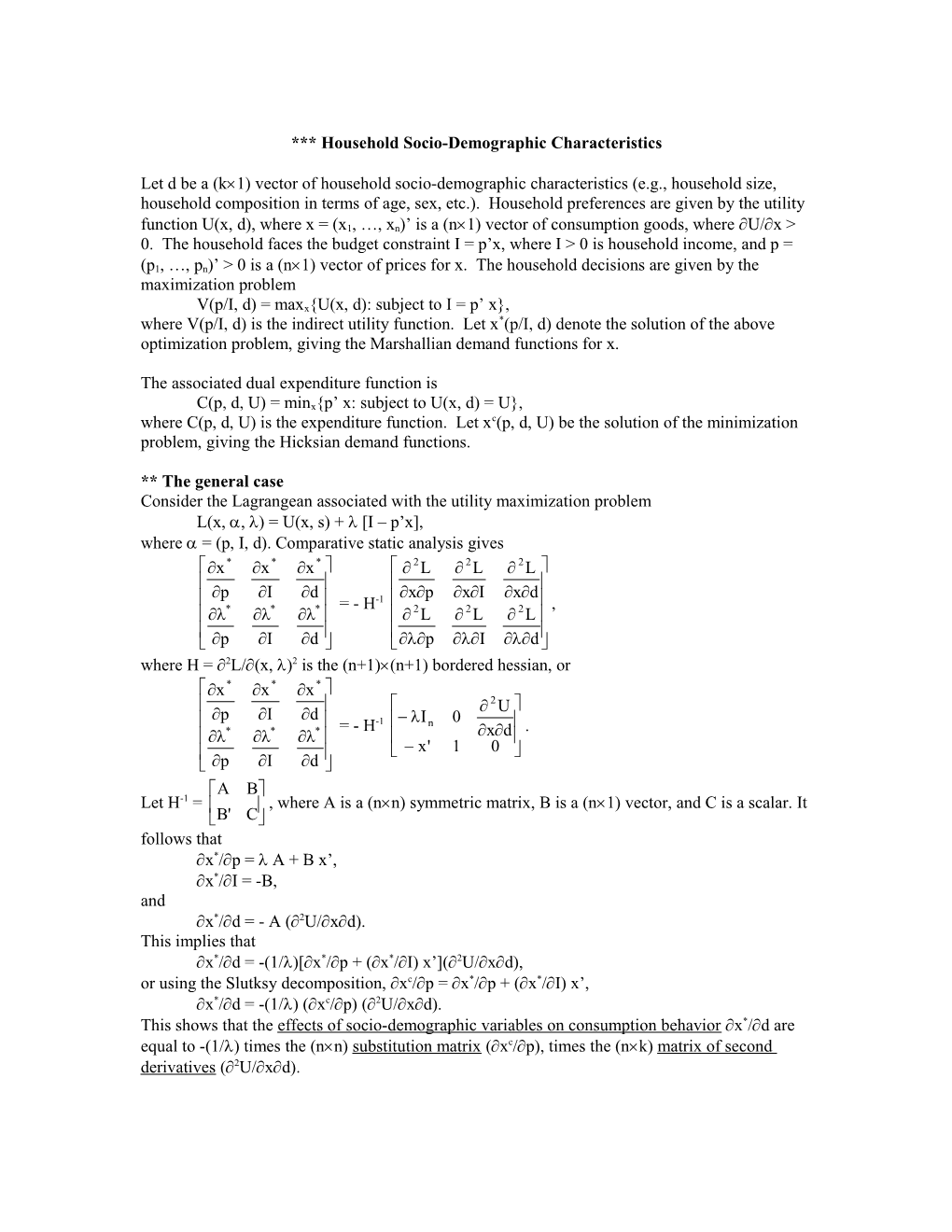
where = (p, I, d). Comparative static analysis gives
= - H-1,
where H = 2L/(x, )2 is the (n+1)(n+1) bordered hessian, or
= - H-1.
Let H-1 = , where A is a (nn) symmetric matrix, B is a (n1) vector, and C is a scalar. It follows that
x*/p = A + B x’,
x*/I = -B,
and
x*/d = - A (2U/xd).
This implies that
x*/d = -(1/)[x*/p + (x*/I) x’](2U/xd),
or using the Slutksy decomposition, xc/p = x*/p + (x*/I) x’,
x*/d = -(1/) (xc/p) (2U/xd).
This shows that the effects of socio-demographic variables on consumption behaviorx*/d are equal to -(1/) times the (nn) substitution matrix (xc/p), times the (nk) matrix of second derivatives (2U/xd).
** Scaling and translating
Consider the special case where
U(x, d)= U[(x1 - T1(d))/S1(d), … , (xn - Tn(d))/Sn(d)],
where T1(d), …, Tn(d) are “translating factors”,
S1(d), …, Sn(d) are “scaling factors”.
* Marshallian demand
Then, household choices are then given by
V(p/I, d) = maxx{U[(x1 - T1(d))/S1(d), … , (xn - Tn(d))/Sn(d)]: p’ x = I}.
Let
Xi = (xi - Ti(d))/Si(d), i = 1, …, n,
or
xi = Xi Si(d) + Ti(d), i = 1, …, n.
It follows that household choices can be alternatively written as
V(p/I, d) = maxX {U(X): subject to pi [Si(d) Xi + Ti(d)] = I},
where X = (X1, …, Xn)’, or
V(p/I, d) = maxX {U(X): subject to pi Si(d) Xi = I - pi Ti(d)}.
This has for solution Xi*[(p1 S1(d))/(I - p’T), … ,(pn Sn(d))/(I - p’ T(d))], i = 1, …, n, where T(d) = (T1(d), …, Tn(d))’ is a (n1) vector of the translating factors. But since xi = Xi Si(d) + Ti(d), if follows that the associated Marshallian demand functions are
xi*(p/I, d) = Si(d) Xi*[(p1 S1(d))/(I - p’T(d)), … ,(pn Sn(d))/(I - p’T(d))] + Ti(d),
i = 1, …, n i = 1, …, n.
Differentiating this expression with respect to d gives
xi*/d = (Si/d) Xi* + Si (Xi*/d) + Ti/d.
Note that
Xi* = (xi* - Ti)/Si,
Xi*/d = (Xi*/ln(pj))(ln(Sj)/d) - (Xi*/I)(pjTj/d).
Thus,
xi*/d = (Si/d)(xi*-Ti)/Si
+ Si(Xi*/ln(pj))(ln(Sj)/d) - Si (Xi*/I)(pjTj/d) + Ti/d.
This decomposes the behavioral effects of socio-demographic variables (xi*/d) into four additive parts: the direct scale effects [(Si/d)(xi*+Ti)/Si], plus the indirect scale effects [Si(Xi*/ln(pj))(ln(Sj)/d)], plus the indirect translating effects [-Si (Xi*/I)(pjTj/d)], plus the direct translating effects (Ti/d). Note that indirect scale effects are proportional to price effects, and that the indirect translating effects are proportional to income effects.
* Hicksian demand
Under scaling and translating, the expenditure function is
C(p, d, U) = minx{p’x: U = U[(x1 - T1(d))/S1(d), … , (xn - Tn(d))/Sn(d)],
which has for solution the Hicksian demand function xc(p, d, U).
Given
Xi = (xi - Ti(d))/Si(d),
or
xi = Xi Si(d) + Ti(d), i = 1, …, n,
the above expenditure function can be written as
C(p, d, U) = minX {pi [Si(d) Xi + Ti(d)]: subject to U = U(X)},
where X = (X1, …, Xn)’, or
C(p, d, U) = pi Ti(d) + minX {pi Si(d) Xi: subject to U = U(X)}
This has for solution Xic[p1 S1(d), … , pn Sn(d), U], i = 1, …, n. But since xi = Xi Si(d) + Ti(d), if follows that the associated Hicksian demand functions are
xic(p, d, U) = Si(d) Xic[p1 S1(d), … , pn Sn(d)] + Ti(d),
i = 1, …, n i = 1, …, n.
Differentiating this expression with respect to d gives
xic/d = (Si/d) Xic + Si (Xic/d) + Ti/d.
Note that
Xic = (xic - Ti)/Si,
Xic/d = (Xic/ln(pj))(ln(Sj)/d).
Thus,
xic/d = (Si/d)(xic-Ti)/Si + Si(Xic/ln(pj))(ln(Sj)/d) + Ti/d.
This decomposes the Hicksian socio-demographic effects (xic/d) into three additive parts: a direct scaling effect [(Si/d)(xic-Ti)/Si], plus an indirect scaling effect [Si(Xic/ln(pj)) (ln(Sj)/d)], plus a translating effect (Ti/d).
* Properties of the expenditure function
Consider the properties of the expenditure function C(p, d, U). Under scaling and translating, using the envelope theorem, we obtain
C(p, d, U)/ln(d) = pi [Ti/ln(d)] + pi [Si/ln(d)] Xic,
= pi [Ti/ln(d)] + pi [Si/ln(d)](xic – Ti)/Si.
This can be written alternatively as
ln(C)/ln(d) = pi [Ti/ln(d)]/C + wic [ln(Si)/ln(d)],
where wic = pi (xic – Ti)/C is an “adjusted cost share” for the i-th commodity, i = 1, …, n.
Now consider a change from in the socio-demographic variables d from dato db. The associated change in the expenditure function is given by
ln[C(p, db, U)/C(p, da, U)] = ln[C(p, db, U)] – ln[C(p, da, U)]
= [ln(C)/ln(d)] dln(d).
Using the above result, it follows that
C(p, db, U)/C(p, da, U) = exp{[ln(C)/ln(d)] dln(d)}.
= exp[{pi [Ti/ln(d)]/C + wic [ln(Si)/ln(d)]} dln(d)].
This shows how the socio-demographic variables d affect the “cost of living” C through the translating factors T and the scaling factors S.
