Teaching Issues and Experiments in Ecology - Volume 7, May 2011

- 1 -

TIEE

Teaching Issues and Experiments in Ecology - Volume 7, May 2011

ISSUES : DATA SET
Global Temperature Change in the 21st Century

Daniel R. Taub1,2 and Gillian S. Graham1

1 - Biology Department, Southwestern University, 1001 East University Ave, Georgetown, TX 78626

2- Corresponding author: Daniel R. Taub ()

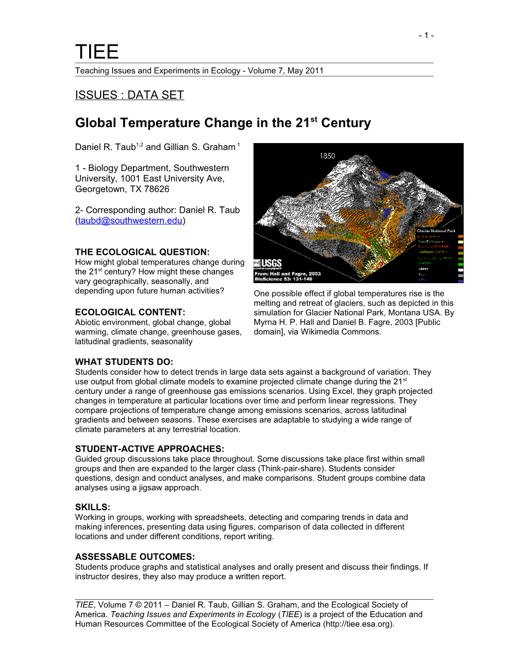
THE ECOLOGICAL QUESTION:

How might global temperatures change during the 21st century? How might these changes vary geographically, seasonally, and depending upon future human activities?

ECOLOGICAL CONTENT:

Abiotic environment, global change, global warming, climate change, greenhouse gases, latitudinal gradients, seasonality

WHAT STUDENTS DO:

Students consider how to detect trends in large data sets against a background of variation. They use output from global climate models to examine projected climate change during the 21st century under a range of greenhouse gas emissions scenarios. Using Excel, they graph projected changes in temperature at particular locations over time and perform linear regressions. They compare projections of temperature change among emissions scenarios, across latitudinal gradients and between seasons. These exercises are adaptable to studying a wide range of climate parameters at any terrestrial location.

STUDENT-ACTIVE APPROACHES:

Guided group discussions take place throughout. Some discussions take place first within small groups and then are expanded to the larger class (Think-pair-share). Students consider questions, design and conduct analyses, and make comparisons. Student groups combine data analyses using a jigsaw approach.

SKILLS:

Working in groups, working with spreadsheets, detecting and comparing trends in data and making inferences, presenting data using figures, comparison of data collected in different locations and under different conditions, report writing.

ASSESSABLE OUTCOMES:

Students produce graphs and statistical analyses and orally present and discuss their findings. If instructor desires, they also may produce a written report.

SOURCES:

Canadian Centre for Climate Modelling and Analysis. Online data repository,

ACKNOWLEDGEMENTS:

We thank the Canadian Centre for Climate Modeling and Analysis for making available the data from their climate models. Dr. Gregory M. Flato provided help in obtaining permission to use this data, and suggested useful approaches for using climate model output. Students in various editions of DRT’s Global Change Biology class provided valuable feedback on these exercises. The editor and two anonymous reviewers provided numerous helpful suggestions.

OVERVIEW OF THE ECOLOGICAL BACKGROUND

Human industrial activity, use of fossil fuels, and land use changes have been leading to increasing emissions and atmospheric concentrations of carbon dioxide and other greenhouse gases (Figure 1). Greenhouse gases are ones that allow electromagnetic radiation (light) at the wavelengths emitted by the sun to pass through to the Earth’s surface, but absorb the radiation that is emitted by the Earth out toward space. In this fashion, they act to heat the atmosphere near the Earth’s surface. Recent increases in the concentrations of these gases, along with increases in temperature, have been the basis for concerns about “global warming.”

Major changes in climate that might result from such increased concentrations of greenhouse gases could of course have profound implications for agriculture, human health, natural resources, and a host of other areas of ecological and social importance. To anticipate these effects, we must first anticipate the details of projected changes in climate. For example, how much warming can be expected to occur over the next century? How would different social, economic, and technological developments affect greenhouse gas emissions and climate change? Would warming be truly global, or vary from location to location? Would warming occur mostly in summer (affecting the prevalence of heat wave, heat damage to crops, etc.), mostly in winter (potentially decreasing the severity of winters, affecting sea ice formation, etc.) or equally in both?

Since these questions concern the future, they cannot be answered directly by empirical observation- unless we are willing to wait decades for the answers. We have only one Earth, so we cannot directly perform experiments with the climate system (other than the one we are inadvertently performing). To make detailed predictions about the future, researchers therefore must rely on perturbing simulated Earths rather than the actual Earth. It would be impossible in a physical simulation (such as a giant globe) to capture the processes in the

Earth’s complex systems in a realistic and meaningful way. Researchers therefore rely on computer simulations that mathematically represent the chemical, physical and biological complexities of global climate systems and how they inter-react and respond to changes in external conditions (such as increasing emissions of CO2 from the burning of fossil fuels).

In practice, there are two major steps to predictions of the effects of future human activities on climate. The first is to predict the quantities of greenhouse gases, particulate matter, and other substances that will be emitted into the atmosphere. The second is to use these estimates of emissions as inputs into models that simulate global climate.

Table 1: Characteristics of Selected Emissions Scenarios. These scenarios represent alternative possibilities for future social and technological change as envisioned by a range of governmental and non-governmental analysts. Adapted from Nakicenovic, N. and R. Swart, eds. (2000). Special Report on Emissions Scenarios (Cambridge, U.K., Cambridge University Press).

Future anthropogenic emissions of gases such as CO2 will vary greatly depending on the rates of human population growth and industrialization and the development and spread of new technologies, such as alternatives to fossil fuels for energy generation. The climate change community has therefore developed a variety of different emissions “storylines” and scenarios that describe alternative versions of future social, economic, and technological changes (Table 1). Each scenario, with its different projections of social, economic and technological changes generates different predicted quantities of emissions and atmospheric concentrations of carbon dioxide (Figure 2) and other greenhouse gases.

Climate simulation models then are used to predict future climates under these different emissions scenarios. Typically, these models divide the surface of the Earth, the ocean and the atmosphere into large spatial cells (Figure 3). Each cell has specified physical properties; for example, a cell in the atmosphere will have a specified temperature, pressure, humidity, etc. In the model, time is simulated in steps; for each step the chemical and physical properties of each cell are updated as the cell receives radiation from the sun and Earth, exchanges energy and materials with adjacent cells, etc. One can use such models to

predict changes in any of these physical and chemical parameters, in any location within the Earth-atmosphere system.

In these exercises, students work with output from simulations of future climates performed using models developed by the Canadian Centre for Climate Modeling and Analysis (CCCma), focusing on near-surface air temperature, a concept familiar through daily weather reports. In doing so, students develop increased understanding of how predictions of future climate are derived, as well as practicing skills in analysis and interpretation of large data sets.

STUDENT INSTRUCTIONS

Background on the data

In these exercises, you will work with output from one set of climate models, created by the Canadian Centre for Climate Modeling and Analysis (CCCma), who have kindly made the results of a number of runs of their models available online. Information on the models can be found on the Models section of the CCCma website ( We will be using data from their third-generation (CGCM3) model. This is the latest model for which they have made available extensive climate predictions over nearly the entirety of the Earth’s surface. We will focus on one parameter, temperature above surface, defined as the air temperature 2 m above the Earth’s surface. This corresponds to the familiar air temperature reported in the daily weather report in newspapers and on TV.

The data you will examine is the mean temperature (°K) for each month over the 100 years (2001-2100), giving a total of 1200 values for the 1200 consecutive months. You are provided these data for the three scenarios described in Table 1 (A1B, A2, and B1) and for a fourth set of conditions representing “Committed” climate change. The “Committed” set of conditions assumes that the composition of the atmosphere remains unchanged at year 2001 values. Therefore, the only climate changes that will occur are those to which the climate system is already committed due to past changes in atmospheric concentrations. The Committed scenario is not intended as a realistic scenario. Instead, it serves as a control for comparison with the other scenarios. By comparing the results of a given scenario with the results under the Committed scenario, one can see how much additional climate change a scenario produces compared to what would be produced if alterations in climate forcing agents were to immediately stop.

For each scenario, we provide data for 19 grid cells in a continuous North-South transect through North America (Figure 4). Your instructor will assign you or your group a latitude or latitudes to work with.

Pre-exercise: Detecting and interpreting trends

In your groups, discuss the following questions to help you consider how you will organize and analyze your data.

1. What would be the best graphical format for presenting the data to illustrate changes (if any) in temperature across the century?

1. How should you organize and analyze the data to determine: 1) whether or not a meaningful trend exists, and 2) how much the temperature has changed (if at all) over the course of the century?

These questions will be discussed with the entire class before you continue on to the exercises below.

Exercises

Exercise 1: Comparison of temperature trends among emissions scenarios

1. Examine the data spreadsheet. Notice the variables that are included, how the data is organized, and the time period it spans.

2. Make a graph showing how summer (July) temperature varies across the 100 years of this study. Begin with the Committed scenario. Only graph the data for your assigned latitude. You will want Year to be the x axis of the graph and Temp to be the y axis. Select these columns (but only for those rows in which the month is July). Use the graphing tools of Excel to create a scatterplot with these values; choose the plot that includes only data points and no connecting lines.

3. Label the axes appropriately, including units. Give the figure an appropriate, detailed title. Since you and the class will be creating a number of different figures, it will be important to have a title that distinguishes among them, including the range of years depicted, the dependent variable, the latitude, and which scenario was used.

4. Insert a trend line (linear regression), including the equation and the R2 value. You can do this by clicking on one of the data points in the figure. This should select the entire series of data points. You can then choose add trend line from the Chart menu (the location of this command may vary with the version of Excel).

5. Note the slope from the trend line equation. Based on this analysis, explain in words how much July temperature changed per year over the time period analyzed.

6. Now, graph the remaining three scenarios for your specific latitude, and add the trend lines to each graph (you will have four total). Note the slope for each equation.

7. Change the scale for the x and y axes for each of your figures. You can do this by clicking on the axis in the finished figure, and then changing the scale values. Set the range of X and Y values for all figures so that they are the same for each figure. This allows for visual comparison of the regression lines.

8. With your group, discuss how temperature has changed in each scenario.

9. Come together as a class so each group can briefly share its findings.

• Are there any patterns as to which scenarios show changes in temperature across the century, or show the greatest change?
• What might differences in projected climate change under these scenarios be due to?
• What might differences among scenarios indicate about future climate change?

Exercise 2: Comparison of temperature change across seasons

1. Repeat Exercise 1, using data from winter (January).

2. Come together as a class for each group to briefly share its findings.

• Does temperature change seem to be more pronounced in one season than in the other?
• What implications might the seasonality of future climate change have for potential impacts (social, ecological, medical, etc.) of climate change?

Exercise 3: Latitudinal Comparisons

1. As a class, devise an approach to share the details of your findings (i.e., the magnitude of temperature change over the century for each analysis you have performed).

2. Once everyone has access to all of the results, each group should examine the results.

• What is the geographic pattern of temperature change? Was it greater at some latitudes than at others? Did it differ between arctic and tropical regions?

3. Discuss these findings as a class.

• What implications might latitudinal patterns of climate change have for the impacts (social, ecological, medical, etc.) of future climate change?

Notes to Faculty

Description of Excel files

• Student dataset (This file contains data for 19 latitudes.) [xlsx]
• Faculty dataset (This file contains data contains data for 19 latitudes, and the faculty file additionally contains the regression slopes and R-squared values for regressions of temperature on year for both January and July for each of the latitudes under the three emissions scenarios in Table 1, and under an additional set of conditions that represent a control set of conditions (the Committed scenario) under which concentrations of greenhouse gases remain constant at year 2000 concentrations.) [xlsx]

Additional Resources

• Student assignment [doc]
• Appendix 1: Downloading additional model output [doc]
• Appendix 2: Kelvin to Celsius Conversion [doc]

Using different, or additional data

The data included in the spreadsheets with this data set is only a tiny fraction of the climate model output available from the Canadian Centre for Climate Modeling and Analysis. Downloading the data and arranging it in a spreadsheet in a useable form is not difficult, but does take a bit of work and some understanding of spreadsheet data manipulation. We have provided detailed instructions on how to do so in Appendix 1. Some of the reasons you may want to download data yourself include:

• To include the geographic location where your institution is located
• To include other geographic areas of particular interest
• To have students examine potential future trends in variables other than air temperature, such as precipitation, soil moisture, snow cover, sea ice cover and thickness, etc.

You also may choose to have students download data for themselves using the instructions in Appendix 1. Some potential advantages of this include:

• Students can choose their own geographic locations of interest
• Students can better understand the source of the data if they download it themselves
• Students can practice and develop skills in data manipulation
• Students can be assigned work to be done outside of class in which they download and analyze data independently

In practice, one of us (DRT) has found that students who have some previous experience with spreadsheets are able to download and process the data for themselves. However, he also has found that students often get stuck if things do not go exactly as planned, due to minor mistakes in the use of the spreadsheet program, variation in the spreadsheet commands from one software release to another, and the like. It is therefore recommended that if students are going to download data for themselves that:

• Students be instructed to register with the CCCma website ahead of time (see Appendix 1)
• The instructor(s) first download and process a set of data using the same equipment and software that the students will use
• If possible, the instructor(s) modify the instructions in Appendix 1, providing details applicable to the particular equipment and software to be used. This may be particularly important for unzipping the compressed files that are downloaded. No instructions on doing this have been provided in Appendix 1, as this process can vary greatly across computer systems.
• The instructor(s) rotate among the students as they are downloading and processing data for the first time, helping to solve problems as they occur

Running the class

For students who have prior experience with Excel, the entire sequence from pre-exercises through exercise three can be easily accomplished within one three-hour lab period. There is often a good deal of heterogeneity among students in their familiarity with Excel. When groups of students finish an exercise quickly, it is usually useful to enlist these students as temporary teaching assistants to help groups that are struggling with spreadsheet procedures.